


Next: 6.3 Determination of Line
Up: 6. Spectroscopy
Previous: 6.1 The Basic Reductions
6.2 Determination of Velocity Dispersion and Radial Velocity
We want to determine the velocity dispersion of the galaxies.
To do this, we make the following assumptions:
- 1.
- The luminosity weighted mean spectrum of the stars in the galaxy
(had they been at rest with respect to each other)
can be well matched by the spectrum of a single template star
(e.g. a K giant).
- 2.
- The line of sight velocity distribution of the stars in the galaxy
(the broadening function) is Gaussian.
Then it is conceptually easy to determine the velocity dispersion:
- a.
- The spectrum of the template star is shifted in wavelength until the
absorption lines in it match those in the galaxy spectrum.
When knowing the (small) velocity of the template star, this gives
the radial velocity of the galaxy.
- b.
- The spectrum of the template star is convolved with
a Gaussian broadening function with dispersion
 ,
and then matched against the galaxy spectrum.
The velocity dispersion is determined as the best fitting value of .
At the same time, the general strength of the absorption lines in the
template star spectrum is also varied in order to get a good fit.
This general line strength relative to the given
template star is not used in our analysis.
It is important that the two spectra are observed with the same instrument,
since the resolution of the spectrograph then cancels out.
,
and then matched against the galaxy spectrum.
The velocity dispersion is determined as the best fitting value of .
At the same time, the general strength of the absorption lines in the
template star spectrum is also varied in order to get a good fit.
This general line strength relative to the given
template star is not used in our analysis.
It is important that the two spectra are observed with the same instrument,
since the resolution of the spectrograph then cancels out.
Specifically, we used the
Fourier fitting method (Franx, Illingworth, & Heckman 1989a),
implemented in a program written by M. Franx.
It calculates the Fourier transforms of the galaxy spectrum
and the template star spectrum,
 and
and
 respectively,
using a common rest frame wavelength interval6.4.
It then iteratively minimizes
respectively,
using a common rest frame wavelength interval6.4.
It then iteratively minimizes
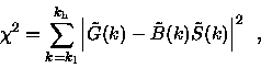 |
(6.1) |
where
 is the Fourier transform of the
Gaussian broadening function.
An analytical expression exists for
as function of
the velocity dispersion ,
the radial velocity, and the relative line strength,
see Sargent et al. (1977).
The iteration solves for all these three variables,
although the radial velocity is not expected to change much.
The Fourier space is used, since a convolution here is a multiplication,
which is computationally faster.
is the Fourier transform of the
Gaussian broadening function.
An analytical expression exists for
as function of
the velocity dispersion ,
the radial velocity, and the relative line strength,
see Sargent et al. (1977).
The iteration solves for all these three variables,
although the radial velocity is not expected to change much.
The Fourier space is used, since a convolution here is a multiplication,
which is computationally faster.
The low and high frequencies in Fourier space
are filtered out before minimizing  .
This is governed by the quantities
.
This is governed by the quantities
 and
and  in Eq. (
![[*]](http://www.astro.ku.dk/Icons/latex2html-96.1/cross_ref_motif.gif) ) above.
We used
) above.
We used
 [= 7/N
  (100 Å)-1] and
 [= 330/N
(2 Å)-1], where
[= 330/N
(2 Å)-1], where
 .
JFK95b used the same values of
and .
.
JFK95b used the same values of
and .
Four K giant template stars were observed a total number of 31 times.
The telescope was attempted moved during the exposures in such a way that the
star would fill the 2
 5 slit in the same way as the galaxies do.
This is needed to get the same resolution for the stars and the galaxies,
since the resolution depends in part on the width of the slit,
and since the seeing is
5 slit in the same way as the galaxies do.
This is needed to get the same resolution for the stars and the galaxies,
since the resolution depends in part on the width of the slit,
and since the seeing is
 2
5.
However, technical problems made this difficult.
Therefore, it was tested which template star observations would give the
lowest velocity dispersions, and the three best,
one observation of each of the stars
HD77236, HD176047, and BD
2
5.
However, technical problems made this difficult.
Therefore, it was tested which template star observations would give the
lowest velocity dispersions, and the three best,
one observation of each of the stars
HD77236, HD176047, and BD
 ,
were actually used in the
Fourier fitting.
,
were actually used in the
Fourier fitting.
From the number of counts in the galaxy spectrum,
the number of counts in the sky spectrum, and
the CCD read-out noise and conversion factor,
the Fourier fitting program calculates
 ,
the number of `effective photons' for the given spectrum.
is defined such that
the signal-to-noise ratio per Å is
,
the number of `effective photons' for the given spectrum.
is defined such that
the signal-to-noise ratio per Å is
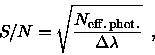 |
(6.2) |
where
 Å is the length of the wavelength interval used
in the fitting.
can also be said to be the
number of photons required to get the S/N actually obtained,
had the sky level and the CCD read-out noise been zero.
The 21 HydraI DFOSC observations have S/N in the range 29.0-73.7,
with a median value of 40.0.
Å is the length of the wavelength interval used
in the fitting.
can also be said to be the
number of photons required to get the S/N actually obtained,
had the sky level and the CCD read-out noise been zero.
The 21 HydraI DFOSC observations have S/N in the range 29.0-73.7,
with a median value of 40.0.
The derived radial velocities were corrected to the heliocentric frame,
 .
The final values of
and
were
taken as the mean of the three determinations.
.
The final values of
and
were
taken as the mean of the three determinations.
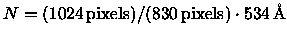
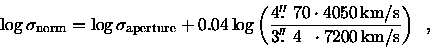
The Fourier fitting was done using an aperture of
2
5  6
59.
2
5 is the width of the slit, and
6
59 (13 pixels) is a user specified length in the spatial direction.
The area of this rectangular aperture is equivalent to a circular
aperture of angular diameter
6
59.
2
5 is the width of the slit, and
6
59 (13 pixels) is a user specified length in the spatial direction.
The area of this rectangular aperture is equivalent to a circular
aperture of angular diameter
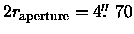 (cf. JFK95b).
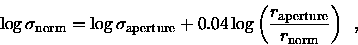
Since E and S0 galaxies have radial gradients in ,
the size of the aperture within which
is measured is of importance.
Following JFK95b,
the measured velocity dispersion,
(cf. JFK95b).
Since E and S0 galaxies have radial gradients in ,
the size of the aperture within which
is measured is of importance.
Following JFK95b,
the measured velocity dispersion,
 ,
was
corrected to an aperture of metric diameter
,
was
corrected to an aperture of metric diameter
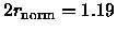 h-1 kpc (H0 = 100 h km/s/Mpc),
corresponding to 3
4 at the distance of the Coma cluster.
The formula used was
h-1 kpc (H0 = 100 h km/s/Mpc),
corresponding to 3
4 at the distance of the Coma cluster.
The formula used was
 |
(6.3) |
where
 is the corrected velocity dispersion.
In practical terms, the calculation was done as
is the corrected velocity dispersion.
In practical terms, the calculation was done as
 |
(6.4) |
where
 and
and
 is the
CMB radial velocity of HydraI and Coma, respectively.
The correction was small, only -0.004.
is the
CMB radial velocity of HydraI and Coma, respectively.
The correction was small, only -0.004.
Next: 6.3 Determination of Line
Up: 6. Spectroscopy
Previous: 6.1 The Basic Reductions
Properties of E and S0 Galaxies in the Clusters HydraI and Coma
Master's Thesis, University of Copenhagen, July 1997

Bo Milvang-Jensen (milvang@astro.ku.dk)